Production

Cratermaker’s production module provides a robust way to compute the production function for craters and projectiles. The production function is defined as the cumulative number of craters greater than a given diameter per unit m² surface area. There are currently two types of production funcitons that are available in the Production class: “neukum” and “powerlaw”. The default production model depends on the value of the target. If the target is one of the inner planets (or Vesta or Ceres), the default will be “neukum”. For all other bodies, it is “powerlaw”. The “neukum” production function comes in three different versions: “moon”, “mars”, or “projectile.” The “projectile” version is used unless the target is either the Moon or Mars. The default Cratermaker target body is the Moon, and therefore the default production function is “neukum” with the “moon” model. We can create a production function object and inspect its values using the following code:

In [1]: from cratermaker import Production

In [2]: production = Production.maker()

In [3]: print(production)
<NeukumProduction>
Generator type crater
Diameter range: 0 m to inf km
N(D) units: N>D(km) per 10⁶ km²
Version: Moon
Valid Time Range: 0 My - 4.500 Gy
Valid Diameter Range: 10.00 m - 1000.0 km

The output shows that by default, the production function is the Neukum model for the Moon, which is described in Neukum, Ivanov, and Hartmann (2001) [1]. It also reports that the “Generator type” is “crater.” A production model can either a crater generator or a projectile generator, which means that the diameter values that are returned from the production function represent either the crater or projectile. The other crater-based model is the Mars version, which is based on the work of Ivanov (2001) [2]. The projectile model is based on the work of Ivanov, Neukum, and Wagner (2001) [3].

The Neukum Moon model has a valid range of ages over which it is valid, which is also reported in the output. The valid range of ages is between 0 and 4.5 Ga, though caution must be used when interpreting ages older than about 3.9 Ga, as these are poorly calibrated. The total crater number density of the most ancient terrains on the Moon correspond to a model age of 4.31 Ga, though the actual crust could potentially be must older than that. Nevertheless, the Neukum model is a well-established and widely used model for inner solar system crater chronology.

The Production class has two primary methods that are used to compute the production function. The first is Production.function(), which computes the expected cumulative number density of craters greater than a given diameter of a surface of a given age. The second is Production.sample(), which samples crater diameters and ages from the production function using Monte Carlo methods.

Production function

Production.function() returns the cumulative size-frequency distribution (CSFD) of craters over a given age range and crater diameter. It takes the following arguments:

• diameter: Crater diameter(s) in units of meters to compute corresponding cumulative number density value.

• time_start: Starting time in units of My relative to the present, used to compute the CSFD. Default is 1.0, corresponding to 1 Ma. Alternatively age can be used as an alias for time_start.

• time_end: Ending time in units of My relative to the present, also used to compute the CSFD. Default is 0.0, which corresponds to the present day.

Example: Using Production.function

For this example, we are going to use Production.function() to find the cumulative number of craters greater than 1 km² to form on a surface in 3 Gy using a power law with a slope of -2.

In [4]: from cratermaker import Production

In [5]: production = Production.maker("powerlaw",slope=-2.0)

In [6]: diameter = 1000.0

In [7]: age = 3000.0

In [8]: n = production.function(diameter=diameter,age=age)

In [9]: print(f"{n*1e6:.2f} D>{diameter*1e-3:.0f} km craters per km² in {age*1e-3:.0f} Gy")
23.65 D>1 km craters per km² in 3 Gy

Example: Plot a power law production function with a slope of -3 for craters 1 m to 100 km over 1 Ga

In [10]: from cratermaker import Production

In [11]: import matplotlib.pyplot as plt

In [12]: import numpy as np

In [13]: fig, ax = plt.subplots()

In [14]: ax.set_xlabel('D (m)')
Out[14]: Text(0.5, 0, 'D (m)')

In [15]: ax.set_ylabel('$\\mathregular{N_{>D}}$')
Out[15]: Text(0, 0.5, '$\\mathregular{N_{>D}}$')

In [16]: production = Production.maker("powerlaw", slope=-3.0)

In [17]: diameters = np.arange(1, 1e6)

In [18]: pf = production.function(diameter=diameters, age=1000.0)

In [19]: ax.loglog(diameters, pf)
Out[19]: [<matplotlib.lines.Line2D at 0x7859f9412710>]

In [20]: plt.show()

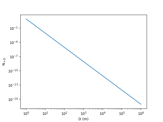
Example: Using Production.age_from_D_N

Production.age_from_D_N() returns the age in My for a given crater number density and diameter. It has the following parameters:

• diameter: Diameter of the crater in m

• cumulative_number_density: Number density of craters per m² surface area greater than the input diameter.

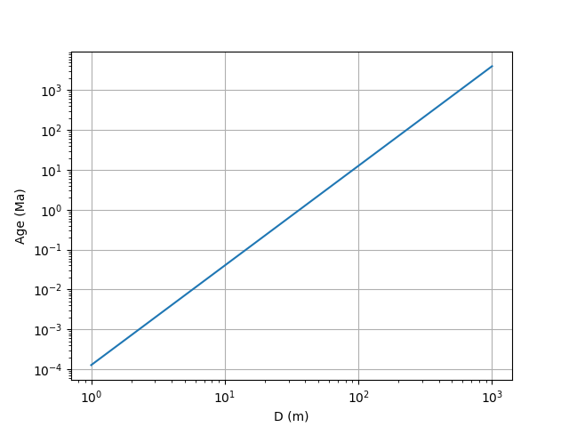
For this example, we are going to use Production.age_from_D_N() to plot the age in Ma for a number density of 10^-6 craters per m² from 1 m to 1 km in diameter.

In [21]: from cratermaker import Production

In [22]: import matplotlib.pyplot as plt

In [23]: import numpy as np

In [24]: production = Production.maker("powerlaw", slope=-2.5)

In [25]: diameters = np.logspace(0, 3)

In [26]: cumulative_number_density = np.full_like(diameters, 1e-6)

In [27]: age = production.age_from_D_N(diameter=diameters, cumulative_number_density=cumulative_number_density)

In [28]: def plot_inv(diameter, age):
   ....:    fig, ax = plt.subplots()
   ....:    ax.set_xlabel('D (m)')
   ....:    ax.set_ylabel('Age (Ma)')
   ....:    ax.loglog(diameters, age)
   ....:    ax.grid(True)
   ....:    return fig
   ....: 

In [29]: fig = plot_inv(diameters, age)

In [30]: plt.show()

Using the Production component in a Simulation

In the above guides we have shown how to use the Production as a standalone object. However, the preferred way of initializing and using this object is as part of a Simulation object, where it is initialized in tandem with all other components in the Cratermaker project. This allows the components to be checked for self-consistency, and streamlines some of the initialization issues. Here we will demonstrate some typical use-cases for Production, including how the valid ranges are dynamically adjusted for the particular Surface and how the Quasi-Monte Carlo functionality allows the user to mix real craters with known properties with randomly-generated craters into a simulation.

Emplace a population of craters drawn from a production function

The Simulation.populate() is used to generate a population of craters drawn from whichever Production component module is loaded into the simulation. You can pass either time interval over which to draw from the production function with either “age” or “time_start” and “time_end”, or you can provide a pair of numbers in the form of (D,N) that represents the production function in the N(D) convention. For instance, to emplace a population of craters corresponding to the production function between 200 My to 100 My before present, you would do:

sim.populate(time_start=200, time_end=100)

The Simulation.populate() method is really meant to be a helper method for the Simulation.run() method, which is used to run a full simulation over a specified time interval. For instance, the Simulation.populate() method does not track the time of emplacement or advance the time interval of the simulation.

Limiting the size range of the production population

When used inside a Simulation, the upper and lower bounds on the sizes of craters returned by Production.function() are set by the resolution of the associated Surface object. The smallest crater that is directly modeled (outside of any subpixel models) is the size of the local face. The largest size is the diameter of the target. These can be adjusted by the user and are access by the smallest_crater and largest_crater attributes.

In [31]: from cratermaker import Simulation

In [32]: sim = Simulation(gridlevel=5)
Creating a new grid
Generating a mesh with icosphere level 5.

In [33]: sim.smallest_crater
Out[33]: 57287.49494015205

In [34]: sim.largest_crater
Out[34]: 3475060.0

Quasi-Monte Carlo craters

For some applications, you may want to specify a predefined population of craters that should be emplaced at a certain time and location along with the random population of craters drawn from the production function. To accomplish this, you can initialize a Simulation object with an argument quasimc_file, which points to either a CSV or NetCDF file containing the information needed to emplace the craters. Alternatively, you When this argumented is passed, the Simulation.run() method will run in “Quasi-Monte Carlo mode”.

Quasi-Monte Carlo mode is a powerful tool that is very flexible. Here we will demonstrate the different ways you can specify craters in the input file and how they affect the behavior of the simulation with a simple donstration using several prominent lunar craters: South Pole-Aitken, Serenitatis, Nectaris, Crisium, Imbrium, Schrödinger, and Orientale. A version of this simulation type with 76 lunar basins and craters is included in the Simuation and Visualization.

First, we we will create a CSV file called “qmc_inputs.csv” and populate it with columns indicating which arguments should be passed to the Crater.maker() function. At a minimum, this requires at least one argument specifying size, such as diameter or projectile_diameter Usually you would include a location as well, which must be specified with “longitude” and “latitude” as separate columns, rather than the typical location tuple that the method call would use. In addition, you typically would provide some indication of when in the simulation you want the crater to form. There are multiple ways to do this.

Specifying an emplacement time

Setting production_time specifies the time when the crater should form along with an optional 1σ standard deviation value. When passing this to Crater.maker() this can be specified as either a single value or a pair of values, where the first value represents the time and the second the standard deviation, both in units of My. The actual time value will be drawn from a normal distribution, unless you only pass a single value to production_time. We will use the age of the Imbrium impact event reported by Nemchin et al. (2021) [4] of 3922±12 My.

In [35]: from cratermaker import Simulation

In [36]: sim = Simulation(gridlevel=5)
Creating a new grid
Generating a mesh with icosphere level 5.

In [37]: qmc_list = []

In [38]: qmc_list.append(sim.Crater.maker(name="Imbrium", diameter=1321e3, location=(341.5, 37), production_time=(3922, 12)))

In [39]: sim.quasimc_craters = qmc_list # This will process the craters and give it a time values bsed on their production metadata

In [40]: print(sim.quasimc_craters[-1])
<Crater>
ID: 1537650261
Name: Imbrium
Diameter: 1321.0 km
morphology_type: complex
transient_diameter: 735.5 km
projectile_diameter: 390.6 km
projectile_mass: 7.0229e+19 kg
projectile_density: 2250 kg/m³
projectile_velocity: 29.50 km/s
projectile_angle: 5.6°
projectile_direction: 218.8°
location (lon,lat): (-18.5000°, 37.0000°)
Production time: 3.922 Gy ± 12.00 My
Emplacement time: 3.928 Gy

The equivalent in a CSV file would be:

qmc_imbrium

name	latitude	longitude	diameter	production_time	production_time_stdev
Imbrium	37	341.5	1321000	3922	12

Note

Always remember that crater chronology model ages are not true ages, especially for the period of time prior to 3900 My bp. It’s best to think of the model age as a way of expressing crater number density (not the other way around), and is subject to change as better calibration data is obtained. Thus a model age of 4310 My bp just means N(20)=999.8 craters per million sq. km. in the Neukum chronology function, which in reality could represent anything from the high 4400s to the mid 4200s. The formation age of the ancient South Pole-Aitken basins, which is stratigraphically the oldest surface feature known on the Moon, has to wait until samples of its melt sheet are returned and dated.

Specifying a production crater number density

Rather than a specific time, you can specify a crater’s “age” by its position on the production function using N(D) convention. This is done by setting the production_ND attribute, which is a tuple of (D, N, N_stdev), where D is the reference diameter in km, N is the cumulative number density of craters per 10⁶ km² greater than D, and N_stdev is the 1σ standard deviation of that number density. Here we will use the N(20) value of the Nectaris basin obtained by Orgel et al. (2020) [5] using the Buffered Non-Sparseness Correction technique, which yielded an N(20)=172±20 per 10⁶ km².

Note

The N(D) convention takes D in units of km, rather than the units of m used when defining craters. To see what unit system is current set, see the N_D_units. Other conventions can be set changing D_conversion_factor and N_conversion_factor.

In [41]: qmc_list.append(sim.Crater.maker(name="Nectaris", diameter=885e3, location=(35.1, -15.6), production_ND=(20, 172, 20)))

In [42]: sim.quasimc_craters = qmc_list # This will process the craters and give it a time values bsed on their production metadata

In [43]: print(sim.quasimc_craters[-1])
<Crater>
ID: 1537650261
Name: Imbrium
Diameter: 1321.0 km
morphology_type: complex
transient_diameter: 735.5 km
projectile_diameter: 390.6 km
projectile_mass: 7.0229e+19 kg
projectile_density: 2250 kg/m³
projectile_velocity: 29.50 km/s
projectile_angle: 5.6°
projectile_direction: 218.8°
location (lon,lat): (-18.5000°, 37.0000°)
Production time: 3.922 Gy ± 12.00 My
Emplacement time: 3.940 Gy

The equivalent in a CSV file would be:

qmc_nectaris

name	latitude	longitude	diameter	production_time	production_time_stdev	production_D	production_N	production_N_stdev
Nectaris	-15.6	35.1	885000			20	172	20
Imbrium	37	341.5	1321000	3922	12

Specifying a sequence constraint

For many craters, it is difficult to constrain their formation time, however we can bracket them stratigraphically relative to other craters. To accomplish this in Cratermaker, we can supply an integer value to the production_sequence attribute. Craters that have a sequence number must form after craters with a lower sequence number. A sequence number can be added to any crater, even if it has another piece of production metadata such as production_time or production_ND, or has none. The only constraint is that at least one crater with the lowest sequence number must have either production_time or production_ND set, otherwise there is no way to determine the earliest time boundary of the sequences.

In this example, will add the basins Fecunditatis and Vaporum. Fecunditatis was determined by Orgel et al. (2020) to have N(90)=10±4 per 10⁶ km². Vaporum is stratigraphically older than Fecunditatis, but younger than South Pole-Aitken (SPA). SPA is stratigraphically the oldest crater on the Moon, so we give it a value of production_sequence of 0. Because it is the oldest, we need an additional constraint. Its absolute formation age is currently not well known. It must be younger than the Moon, so is likely less than 4500 My. There are materials older than about 4250 My that are attributed to basins other than SPA, so it is likely older than that. We will therefore constrain it to an N(20)=999 per 10⁶ km², which is the value of the production function at 4310 My bp. Fecunditatis is younger than Vaporum, so we give it a sequence number of 10, and Vaporum gets a sequence number of 5, and no other constraints. We can also add sequence constraints to Nectaris and Imbrium.

Our input file for this set of craters would look like this:

qmc_selected_basins

name	latitude	longitude	diameter	production_time	production_time_stdev	production_D	production_N	production_N_stdev	production_sequence
South Pole-Aitken	-53	191	2400000			20	999		0
Vaporum	14.2	3.1	410000						5
Fecunditatis	-4.6	52	690000			90	10	4	10
Nectaris	-15.6	35.1	885000			20	172	20	40
Imbrium	37	341.5	1321000	3922	12				100

In [44]: sim = Simulation(gridlevel=5, quasimc_file="qmc_selected_basins.csv", ask_overwrite=False)

In [45]: for crater in sim.quasimc_craters:
   ....:     N20 = sim.production.function(diameter=20e3, age=crater.time) * 1e12
   ....:     N64 = sim.production.function(diameter=64e3, age=crater.time) * 1e12
   ....:     n20text = f"N(20) = {N20:.1f}"
   ....:     n64text = f"N(64) = {N64:.1f}"
   ....:     stext = f"{crater.production_sequence}" if crater.production_sequence is not None else "-"
   ....:     print(f"{crater.name:22}: {crater.time:.1f} My {n20text:15} {n64text:14} {stext:5}")
   ....: 
South Pole-Aitken     : 4309.9 My N(20) = 999.0   N(64) = 97.9   0    
Vaporum               : 4267.4 My N(20) = 745.7   N(64) = 73.1   5    
Fecunditatis          : 4185.9 My N(20) = 426.8   N(64) = 41.8   10   
Nectaris              : 4037.0 My N(20) = 156.1   N(64) = 15.3   40   
Imbrium               : 3932.6 My N(20) = 78.9    N(64) = 7.7    100  

Note

The numerical value of the production_sequence is only important if there are no other production metadata constraints, such as in the Vaporum example. In that case, the N(1) range corresponding to the sequence is an interpolation between bordering sequences. So in the above case, Vaporum’s nominal “age” (in N(1) value) would be determined by extrapolating the N(1) values of craters with sequence 10 (Fecunditatis) and sequence 0 (SPA). With a value of 5, Vaporum would have a nominal N(1) value exactly in the middle, though its actual value will still be drawn from a normal distribution.

Adjusting the automatic crater size limit

By default, when a list of craters with production metadata is loaded into quasimc_craters, the upper range of the randomly-generated craters is adjusted so that it is limited to the size of the smallest crater in the quasimc_craters list. However, sometimes this is not desirable. For instance, suppose we want to add Copernicus to our list. If we didn’t change the range of craters, this would mean that the simulation would never create random craters larger than the 96 km diameter of Copernicus. We can therefore adjust the largest_crater attribute as needed.

qmc_with_copernicus

name	latitude	longitude	diameter	production_time	production_time_stdev	production_D	production_N	production_N_stdev	production_sequence
South Pole-Aitken	-53	191	2400000			20	999		0
Vaporum	14.2	3.1	410000						5
Fecunditatis	-4.6	52	690000			90	10	4	10
Nectaris	-15.6	35.1	885000			20	172	20	40
Imbrium	37	341.5	1321000	3922	12				100
Copernicus	9.6209	339.9214	96070	800.0	15				200

In [46]: sim.quasimc_file="qmc_with_copernicus.csv"

In [47]: print(f"Largest random crater: {sim.largest_crater * 1e-3:.1f} km")
Largest random crater: 410.0 km

# Now set the largest crater
In [48]: sim.largest_crater = 200e3

In [49]: print(f"Largest random crater: {sim.largest_crater * 1e-3:.1f} km")
Largest random crater: 200.0 km

More Production examples

See more examples at Production Functions and Monte Carlo Utilities and Simuation and Visualization.

References

[1]

Neukum, G., Ivanov, B.A., Hartmann, W.K., 2001. Cratering Records in the Inner Solar System in Relation to the Lunar Reference System. Space Science Reviews 96, 55-86. doi:10.1023/A:1011989004263

[2]

Ivanov, B.A., 2001. Mars/Moon Cratering Rate Ratio Estimates. Space Science Reviews, 96, 87-104. doi:10.1023/A:1011941121102

[3]

Ivanov, B.A., Neukum, G., Wagner, R., 2001. Size-Frequency Distributions of Planetary Impact Craters and Asteroids, in: Collisional Processes in the Solar System. Springer Netherlands, Dordrecht, pp. 1-34. doi:10.1007/978-94-010-0712-2_1

[4]

Nemchin, A.A., Long, T., Jolliff, B.L., Wan, Y., Snape, J.F., Zeigler, R., Grange, M.L., Liu, D., Whitehouse, M.J., Timms, N.E., Jourdan, F., 2021. Ages of lunar impact breccias: Limits for timing of the Imbrium impact. Geochemistry 81, 125683. doi:10.1016/j.chemer.2020.125683

[5]

Orgel, C., Michael, G., Fassett, C.I., van der Bogert, C.H., Riedel, C., Kneissl, T., Hiesinger, H., 2018. Ancient Bombardment of the Inner Solar System: Reinvestigation of the “Fingerprints” of Different Impactor Populations on the Lunar Surface. J. Geophys. Res. 123, 748–762. doi:10.1002/2017JE005451