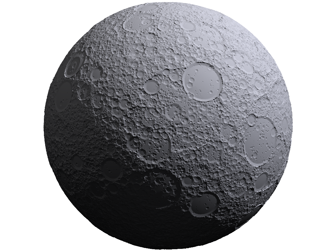
Simulation

Simulation#

The Simulation class manages the evolution of cratered planetary surfaces. It contains components such as target bodies, impactor distributions, and emplacement to simulate crater formation over time.

A Simulation instance can be initiated with keyword arguments specifying the various component models to be used in the simulation. These components include:

Any valid arguments for these components can be passed directly to the Simulation constructor, otherwise default values will be used (see the guide for Default Behavior).

Creating craters and populations of craters#

The Simulation class has set of core methods that can be used to generate craters, using the requested (or default) Production and Morphology components onto the requested Surface component. These are emplace(), populate(), and run(). Each successive method makes use of the others (that is, populate() calls emplace() on the craters in generates, and run() calls populate() for each interval of time in the simulation). We will discuss each of these in turn:

Emplace one or more specific craters#

The emplace() is used to emplace one or more craters onto a surface. The arguments are either the parameters that you would pass to Crater.maker() to generate a single crater, a single Crater object, or a list of Crater objects. So for instance, you can emplace a single 300 km crater onto a random location on a surface, you would do:

from cratermaker import Simulation

sim = Simulation()
sim.emplace(diameter=300e3)

To place 3 craters onto the surface, you could do the following:

from cratermaker import Crater

craters = [Crater.maker(diameter=d) for d in [100e3, 200e3, 300e3]]
sim.emplace(craters)

Emplace a population of craters drawn from a production function#

The next level of methods is populate(), which is used to generate a population of craters drawn from whichever Production component module is loaded into the simulation. The arguments for this method are the same as those for populate(), which can either be the time interval over which to draw from the production function, or a pair of diameter/number values that specify the position in the production function to draw from. For instance, to emplace a population of craters corresponding to the production function between 200 My to 100 My before present, you would do:

sim.populate(time_start=200, time_end=100)

The populate() method is really meant to be a helper method for the run() method, which is used to run a full simulation over a specified time interval. For instance, the The populate() method does not track the time of emplacement or advance the time interval of the simulation.

Running a Simulation#

Once a Simulation instance has been created, the simulation can be run using the run() method. This method requires an age argument specifying the duration of the simulation in million years (My).

The following example configures a simulation targeting the Moon and runs it for 4 Gy, then we plot the number of true emplaced (countable) craters as well as the number of observed craters that the crater counting algorithm has determined are observable. To speed up the example, we have reduced the resolution of the surface grid from the default value of 8 to 6 using the gridlevel argument.

In [1]: from cratermaker import Simulation

In [2]: sim = Simulation(target="Moon", gridlevel=6, rng_seed=7636830)
Creating a new grid
Generating a mesh with icosphere level 6.

In [3]: sim.run(age=4000)

In [4]: print(f"Number of true emplaced craters: {sim.n_emplaced}")
Number of true emplaced craters: 23

In [5]: print(f"Number of observed craters: {sim.n_observed}")
Number of observed craters: 23

Note

You may notice that the number of craters emplaced during the Simulation is much larger than the value of true emplaced craters given by sim.n_emplaced. This is because the Counting object only tracks craters that are potentially countable. Most of the craters that are emplaced during a simulation are too small to be reliably counted, so while they are still modify the surface, they are not tracked by the counting system.

Multi-interval Simulations#

The run() method can also be used to run a simulation in multiple intervals, which is useful for tracking the evolution of the cratered surface over time. To do this, you can pass either the time_interval or ninterval arguments. These two arguments are mutually exlusive, as they divide up the simulation in different ways.

Equal time intervals#

When passing the time_interval argument, the simulation is divided up into equal intervals of time. Depdning on which production function is enabled (see Production) the rate of cratering may be different at different points in time. For instance, in the default Neukum production function for the Moon, the cratering rate is significantly hire prior to about 3 Ga before present, so a simulation that spans these early times will produce more craters in the early time intervals than in the later ones.

In the example below, we demonstrate how a simulation with time_interval=1000 would behave by drawing the numbers of craters larger than 10 km between equal time intervals on the surface of the Moon.

In [6]: from cratermaker import Production, Target

In [7]: target = Target.maker("Moon")

# We'll pass a rng_seed value so that the example always gives the same answer.
In [8]: production = Production.maker("neukum", target=target, rng_seed=2029821)

In [9]: diameters1, _ = production.sample(time_start=4000, time_end=3000, diameter_range=(10e3, 10000e3), area=target.surface_area, return_age=False)

In [10]: print(f"Number of craters emplaced between 4000 Ma and 3000 Ma: {len(diameters1)}")
Number of craters emplaced between 4000 Ma and 3000 Ma: 10116

In [11]: diameters2, _ = production.sample(time_start=3000, time_end=2000, diameter_range=(10e3, 10000e3), area=target.surface_area, return_age=False)

In [12]: print(f"Number of craters emplaced between 3000 Ma and 2000 Ma: {len(diameters2)}")
Number of craters emplaced between 3000 Ma and 2000 Ma: 150

In [13]: print(f"Ratio of craters emplaced between 4000-3000 Ma to 3000-2000 Ma: {len(diameters1) / len(diameters2)}")
Ratio of craters emplaced between 4000-3000 Ma to 3000-2000 Ma: 67.44

In this example the first billion years (from 4000 Ma to 3000 Ma before present) of a simulation using this production function would produce almost 70 times more craters than the second billion years (from 3000 Ma to 2000 Ma before present).

Equal number of craters per interval#

When passing the ninterval argument, the simulation is divided up into intervals that each contain approximately the same number of emplaced craters. The true number of craters produced in each interval won’t be exactly the same because the number of craters is goverened by the Poisson distribution.

In the example below, we will demonstrate how a simulation with equal number intervals would behave by sampling an expected number of 100 craters larger than 10 km:

In [14]: diameters1, _ = production.sample(diameter_number=(10e3, 100), diameter_range=(10e3, 10000e3), area=target.surface_area, return_age=False)

In [15]: print(f"Number of craters in sample 1: {len(diameters1)}")
Number of craters in sample 1: 103

In [16]: diameters2, _ = production.sample(diameter_number=(10e3, 100), diameter_range=(10e3, 10000e3), area=target.surface_area, return_age=False)

In [17]: print(f"Number of craters in sample 2: {len(diameters2)}")
Number of craters in sample 2: 101

As can be seen, the toltal numbers of craters is somewhat different in each sample, but they are both within the expected variability of the Poisson distribution for a mean of 100 craters in the sample.

Save Actions#

The Simulation class has a “save_actions” parameter that can be set by any component class and is used to invoke specific method calls on the component when its .save() method is called. This is useful to trigger specific postprocesing actions, like plotting or exporting, at the end of each interval of a Simulation run. The save_actions attribute takes a dictionary where each key is a valid method that can be called on the component (such as “plot”, “export”, “show3d”, etc.) and the values are a dictionary of arguments that you would pass to that method. Currently, Cratermaker has a default save action that will run the plot command, which will get called at the beginning of a run in order to save the initial condiations, and at the end of each interval of a multi-interval run or at the end of the simulation’s run command.

In [18]: sim = Simulation(gridlevel=4)
Creating a new grid
Generating a mesh with icosphere level 4.

In [19]: print(sim.save_actions)
[{'plot': {'plot_style': 'hillshade', 'show': False, 'save': True}}]

If you wanted to automatically export the crater count data to Spatial Crater Count (SCC) format that can be read in by Craterstats, you could set the following save actions:

from cratermaker import Simulation

sim = Simulation()
sim.counting.save_actions = [{"export": {"driver": "SCC"}}]
sim.run(time_start=3000, time_interval=1000)

You can also can have multiple save actions that use the same method, but with different arguments. So for instance, suppose you want to generate a plot with the craters overlaied onto the hillshade of the standard suface plot. You could set up a simulation like this:

from cratermaker import Simulation

sim = Simulation(
    surface="hireslocal",
    local_location=(0, 0),
    pix=10.0,
    local_radius=2500.0,
    ask_overwrite=False,
    reset=True,
)
# Add an extra plot command on top of the default one for Simulation so that we plot both the standard hillshade but also one with the craters overlaid.
sim.add_save_action({"plot": {"include_counting": True, "show": False, "save": True}})

# Also export the craters in SCC format at the end of each interval as part of the Counting object's save_actions.
sim.counting.add_save_action({"export": {"driver": "SCC"}})
sim.run(age=3540.0, time_interval=10.0)

More Examples#

More detailed component examples are provided in the Gallery section.