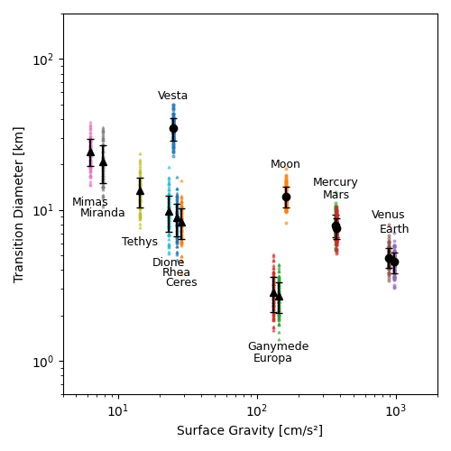
The simple-to-complex transition diameter

By David Minton

This example demonstrates how to use the Scaling class to calculate the simple-to-complex transition diameter as a function of surface gravity bodies using the Monte Carlo scaling model. Because the scaling model is non-deterministic, we sample each body 100 times to get a distribution of transition diameters. We plot the mean and standard deviation of the transition diameter is plotted for each body, showing results that resemble Fig. 7 of Schenk et al. (2021) [1].

References

[1]

Schenk, P., Castillo-Rogez, J., Otto, K.A., Marchi, S., O’Brien, D., Bland, M., Hughson, K., Schmidt, B., Scully, J., Buczkowski, D., Krohn, K., Hoogenboom, T., Kramer, G., Bray, V., Neesemann, A., Hiesinger, H., Platz, T., De Sanctis, M.C., Schroeder, S., Le Corre, L., McFadden, L., Sykes, M., Raymond, C., Russell, C.T., (2021) Compositional control on impact crater formation on mid-sized planetary bodies: Dawn at Ceres and Vesta, Cassini at Saturn. Icarus 359, 114343. doi: 10.1016/j.icarus.2021.114343

import matplotlib.pyplot as plt
import numpy as np

from cratermaker import Scaling

silicate_bodies = ["Vesta", "Moon", "Mercury", "Mars", "Earth", "Venus"]
ice_bodies = [
    "Mimas",
    "Miranda",
    "Tethys",
    "Dione",
    "Rhea",
    "Ceres",
    "Ganymede",
    "Europa",
]

fig, ax = plt.subplots(figsize=(5, 5))
ax.set_xscale("log")
ax.set_yscale("log")
ax.set_xlabel("Surface Gravity [cm/s²]")
ax.set_ylabel("Transition Diameter [km]")
ax.set_xlim((4, 2000))
ax.set_ylim((0.6, 200))
color_index = 0
label_color_map = {}
nsamples = 100
bodies = silicate_bodies + ice_bodies
for body in bodies:
    scaling = Scaling.maker(target=body)
    Dt_list = []
    g_list = []
    for _ in range(nsamples):
        Dt_list.append(scaling.transition_diameter * 1e-3)
        g_list.append(scaling.target.gravity * 100)
        scaling.recompute()

    Dt_arr = np.array(Dt_list)
    g_arr = np.array(g_list)
    g_mean = np.mean(g_arr)
    Dt_mean = np.mean(Dt_arr)
    Dt_std = np.std(Dt_arr)
    if body == "Europa":
        label_offset = 0.6 * Dt_mean
    elif body == "Ceres":
        label_offset = 0.57 * Dt_mean
    elif body == "Rhea":
        label_offset = 0.53 * Dt_mean
    elif body == "Mercury" or body == "Venus":
        label_offset = 0.75 * Dt_mean
    else:
        label_offset = 0.5 * Dt_mean

    if body in silicate_bodies:
        marker = "o"
        va = "bottom"
        y_text = Dt_mean + label_offset
    else:
        marker = "^"
        va = "top"
        y_text = Dt_mean - label_offset

    ax.plot(g_arr, Dt_arr, marker, markersize=2, alpha=0.5, label=f"{body} samples")
    ax.errorbar(
        g_mean,
        Dt_mean,
        yerr=Dt_std,
        fmt=marker,
        color="k",
        capsize=3,
        label=f"{body} mean",
    )
    ax.text(g_mean, y_text, body, fontsize=9, ha="center", va=va)

plt.tight_layout()
plt.show()