Surface

Cratermaker’s Surface component is used to represent target body’s topography and other properties of its surface. Its prupose is to handle surface-related data by providing methods for setting elevation data, and calculating surface-related questions. The Surface class number of attributes and methods that allow the user to perform various operations on the surface. Every Surface object contains the following basic attributes:

• target: The Target that the surface is associated with. The default target is “Moon.”

• radius: The radius of the target body in meters. This is a convenience attribute that retrieves the radius from the Target object.

• smallest_length: The smallest length scale that the surface can resolve. This is used for determining minimum elevation changes, such as when ejecta deposits are added to the surface. It is set when the surface is created.

• gridtype: The type of surface grid that is being used. This will be one of “icosphere,” “arbitrary_resolution,” “hireslocal,” or “datasurface,” depending on how it was created.

• output_dir: The directory where the surface data files are stored.

• uxds, uxgrid: The UxArray dataset and grid object used to represent the surface mesh (see the next section for more details).

The UxArray-based surface mesh

The surface of a celestial body in Cratermaker is represented as a sphere that has been discretized as an unstructured polygonal mesh using the UxArray package. UxArray provides a rich set of tools for representing unstructured mesh geometry and data associated with the mesh, through their UxDataset and associated Grid. The surface mesh is composed of faces, nodes, and edges, where each face is a polygonal shape defined by its nodes. The faces are connected to each other through edges, and the nodes are the points in space that define the corners of the faces. A simple diagram showing the relationship between faces, nodes, and edges is shown below:

In the above image, show a single face with 6 nodes and 6 edges, surrounded by 6 neighboring faces. Each face, node, and edge is identified with an integer index. A Surface object contains a number of attributes that represent the mesh geometry and connectivity, such as:

• n_face: The number of faces in the surface mesh.

• n_node: The number of nodes in the surface mesh.

• n_edge: The number of edges in the surface mesh.

• face_area : An array that contains the area of each face in m²

• face_size : The “effective” size of each face, which is defined as the square root of the area of each face in meters.

• pix : The estimated effective size of the faces in meters.

• pix_mean : The mean effective size of the faces in meters. This is the average of the face_size array.

• pix_std : The standard deviation of the effective size of the faces in meters. This is the standard deviation of the face_size array.

• pix_max : The maximum effective size of the faces in meters. This is the maximum value of the face_size array.

• pix_min : The minimum effective size of the faces in meters. This is the minimum value of the face_size array.

• face_x, face_y, face_z: Arrays that contain the x, y, and z coordinates of the center of each face in Cartesian coordinates.

• node_x, node_y, node_z: Arrays that contain the x, y, and z coordinates of each node in Cartesian coordinates.

• face_lon, face_lat: Arrays that contain the longitude and latitude of the center of each face in degrees.

• node_lon, node_lat: Arrays that contain the longitude and latitude of each node in degrees.

• Variables of uxds: Any variable that is stored inside the UxDataset associated with the surface can be accessed as an attribute of Surface. For instance, the face and node elevations arrays can be retrieved by calling Surface.elevation_face and Surface.elevation_node, respectively, where these variables are stored in the UxDataset as “elevation_face” and “elevation_node”. This is done through the __getattr__ method of Surface, which checks if the requested attribute is a variable in the UxDataset and returns its data if it is.

Note

The mesh itself remains static inside Cratermaker, and so the elevations are only applied to the mesh when it is visualized.

Many of the above attributes are based on similar once found in UxArray, though some are modified to be more useful for Cratermaker’s purposes. For instance, the face_area attribute is computed using the true dimensions of the surface, rather than assuming a unit sphere, which is how UxArray computes it by default. You can access the underlying UxArray structures through the uxds and uxgrid properties.

Mesh connectivity

Many of the functions within Cratermaker require knowledge of the connectivity between faces, nodes, and edges. The Surface object contains several attributes that represent this connectivity:

• face_face_connectivity: An array that contains the faces that surround each face.

• face_node_connectivity: An array that contains the nodes that are associated with each face.

• face_edge_connectivity: An array that contains the edges that are associated with each face.

• node_face_connectivity: An array that contains the faces that are associated with each node.

• edge_node_connectivity: An array that contains the nodes that are associated with each edge.

• edge_length: An array that contains the length of each edge in meters.

• edge_face_distance: An array that contains the distance between the centers of the two faces that saddle each edge in meters.

As an example of how these are structured, take the diagram shown above of a single face with 6 nodes and 6 edges. The following table shows the connectivity arrays for that face:

face_face_connectivity[0] = [1, 2, 3, 4, 5, 6]
face_node_connectivity[0] = [0, 1, 2, 3, 4, 5]
face_edge_connectivity[0] = [0, 1, 2, 3, 4, 5]
node_face_connectivity[0:6] = [[1, 0, 2], [0, 3, 2], [0, 4, 3], [5, 4, 0], [6, 5, 0], [6, 0, 1]]
edge_node_connectivity[0:6] = [[0, 1], [0, 2], [0, 3], [0, 4], [0, 5], [0, 6]]

In the next section we will describe the different types of surfaces that can be created in Cratermaker, and how they are used.

Surface Types

Like all Cratermaker components, a Surface object is instantiated with a special factory method called Surface.maker(), along with arguments that control how the Surface is created. There are currently three different surface types of surface implementations that can be chosen by the user, which are selected by passing the surface argument to the Surface.maker() method. The available surface types are:

• "icosphere": This is the default surface type, which generates a uniform grid configuration with polygonal faces that will be subdivided by the input value for the gridlevel argument. The icosphere surface will have the most uniform face sizes, but is limited to a few resolutions. It is best suited for general use and is the default surface type.

• "arbitrary_resolution": This surface type allows the user to define the approximate size of the faces of the grid using the pix argument. It creates a uniform grid configuration but allows for more control over the sizes of the faces. The faces on this surface will be more irregular in shape, making it less ideal for some applications, but it is useful when specific face sizes are needed.

• "hireslocal": This surface type is used for modeling a small local region at high resolution. It requires the pix, local_radius, local_location, and superdomain_scale_factor arguments. The local region is the “primary” surface being modeled, and the superdomain is simply a source for distal ejecta from large far away craters. This surface type is useful for applications that require high resolution in a small area, but still allows for global processes to affect the small local area.

• "datasurface": This surface type is based on "hireslocal" but will construct a surface and initialize it based on a digital elevation model (DEM). When using the Moon as a target body, can fetch DEM data from the NASA PDS automatically, and only requires a minimum of the local_location and local_radius arguments. By default, it will find data file that contains approximately \(10^6\) faces. Passing an optional argument pix will override this default behavior and it will attempt to find a DEM file that comes closest to matching the requested pixel size. Optionally, the user can also pass in one or more file paths or URLs to DEM files using the dem_file_list argument. Like “hireslocal,” this surface will contain a local region and a global superdomain. The superdomain will be initialized using a low resolution global DEM, or optionally a file path or URL to a DEM file can be passed in using the superdomain_dem_file argument.

The following sections will describe each of these surface types in more detail, including how to create them and their specific attributes and methods.

Icosphere

The default Surface is “icosphere,” which consists of a uniform grid configuration with polygonal faces that are be subdivided by the input value for the gridlevel argument. The number of faces and nodes of the icosphere is determined by the formulas \(N_{face} = 10\times4^{gridlevel}+2\) and \(N_{node} = 20\times4^{gridlevel}\). The Surface object contains an attribute called pix, which is the value of the “effective pixel size” in meters, where \(pix=\sqrt{\left<Area_{face}\right>}\). The following table shows the relationship between the grid level, the number of faces and nodes, and the effective pixel size for a default target of the Moon:

gridlevel	n_face	n_node	pix (for Moon target)
5	10242	20480	60.8 km ± 2.42 km
6	40962	81920	30.4 km ± 1.25 km
7	163842	327680	15.2 km ± 634 m
8	655362	1310720	7.60 km ± 319 m
9	2621442	5242880	3.80 km ± 160 m

Though it is limited to a few resolutions, the icosphere surface will have the most uniform face sizes. Lower values of gridlevel will result in fewer but larger face sizes, which can be computed quickly but will not resolve detail well. Higher values of gridlevel will result in more faces with smaller areas, which will resolve detail better but will take longer to generate and use, and will consume more memory. The default value is 8, and we recommend keeping gridlevel to between ~7-9. Also, keep in mind that the value of pix in the table above is computed for the Moon, and will vary for other targets.

In [1]: from cratermaker import Surface

In [2]: surface=Surface.maker()
Creating a new grid
Generating a mesh with icosphere level 8.

In [3]: print(surface)
<IcosphereSurface>
Target: Moon
Grid File: surface/grid.nc
Number of faces: 655362
Number of nodes: 1310720
Grid Level: 8
Effective pixel size: 7.602 km +/- 319.2 m

This is equivalent to:

In [4]: surface=Surface.maker(surface='icosphere', gridlevel=8, target='Moon')
Creating a new grid
Generating a mesh with icosphere level 8.

In [5]: print(surface)
<IcosphereSurface>
Target: Moon
Grid File: surface/grid.nc
Number of faces: 655362
Number of nodes: 1310720
Grid Level: 8
Effective pixel size: 7.602 km +/- 319.2 m

Arbitrary Resolution

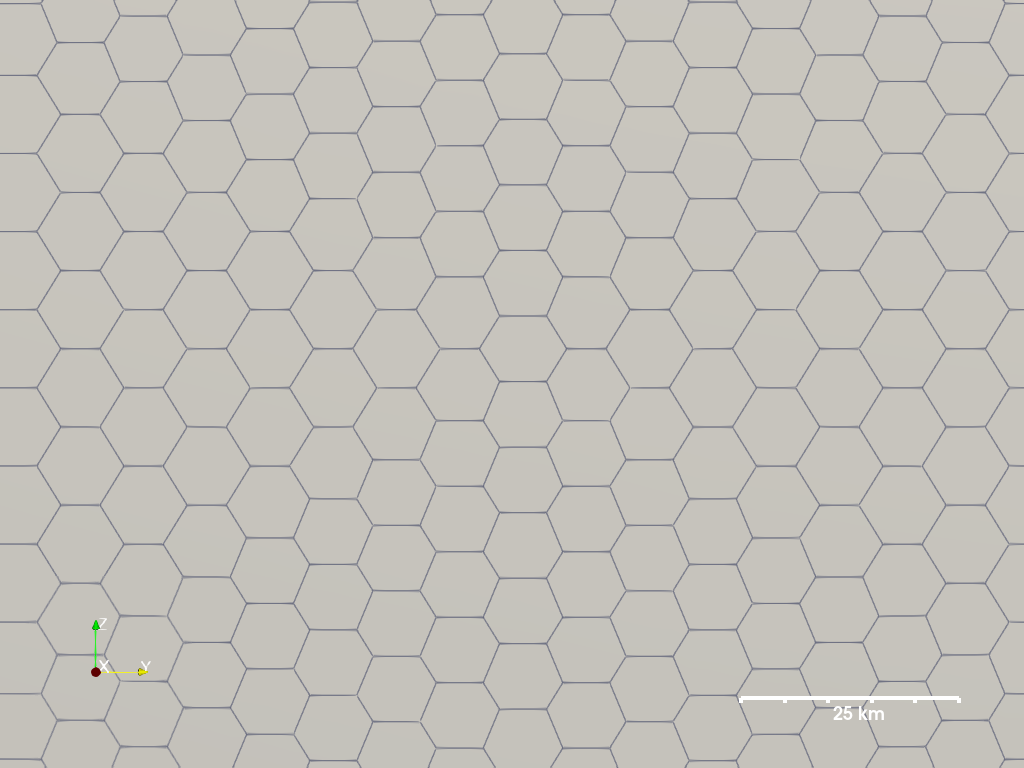
While the "icosphere" surface generates the most regular grids, it is limited to only a few fixed face sizes. If you wish to have more control over the sizes of your faces, you can use the "arbitrary_resolution" surface type instead of “icosphere.” The "arbitrary_resolution" surface takes an argument called pix, which sets the approximate size of the faces of the grid. The value of pix is given in units of meter, and it is defined such that the area of each face will on average be \(pix^2\). For instance, suppose we want to create a surface representation of planet Mercury with a resolution of 20 km per face (shown in the figure above):

In [6]: surface=Surface.maker(surface="arbitrary_resolution", target='Mercury', pix=20e3)
Creating a new grid
Generating a mesh with uniformly distributed faces of size ~20.00 km.

In [7]: print(surface)
<ArbitraryResolutionSurface>
Target: Mercury
Grid File: surface/grid.nc
Number of faces: 186945
Number of nodes: 373886
Effective pixel size: 20.00 km +/- 332.8 m

The arbitrary resolution grid is similar to the icosphphere grid in that the surface will be discretized into approximately equal-sized faces. Unlike the icosphere, the faces on the surface will be more irregular in shape, making it less ideal.

High Resolution Local

In many application of Cratermaker, it is useful to model a small local region at high resolution. This can be done with the "hireslocal" Surface type. This Surface requires the following 4 arguments:

• pix: The pixel size in meters within the high resolution local region.

• local_radius: The radius of the local region in meters.

• local_location: The center of the local region in degrees, given as a tuple of (longitude, latitude).

• superdomain_scale_factor: A scale factor that determines how much larger the faces will be at the antipode of the local region.

Note

When used as part of a Simulation, the superdomain_scale_factor can be omitted. It is computed using the Simulation’s production and morphology models in order to compute the sizes of faces in the superdomain as a function of distance from the local region boundary.

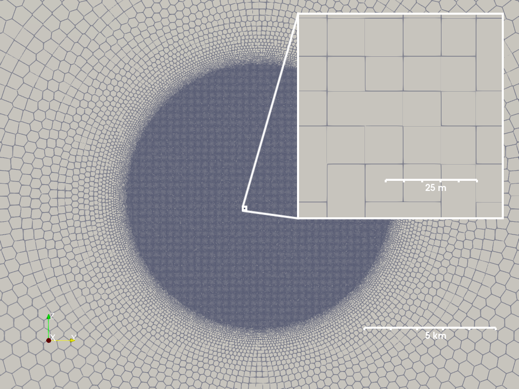
For instance, suppose we want to generate a high resolution local grid on the Moon with a resolution of 10 m per pixel, with a high resolution region radius of 5 km, centered at the equator and prime meridian (0° longitude, 0° latitude), and a superdomain scale factor of 10,000:

In [8]: surface=Surface.maker("hireslocal", pix=10.0, local_radius=5e3, local_location=(0, 0), superdomain_scale_factor=10000)
Generating a new grid.
Creating a new grid
Center of local region: (0.0, 0.0)
Radius of local region: 5.000 km
Local region pixel size: 10.00 m
Generated 782071 points in the local region.
Generated 316659 points in the superdomain region.

In [9]: print(surface)
<HiResLocalSurface>
Target: Moon
Grid File: surface/grid.nc
Number of faces: 1098642
Number of nodes: 2197280
Local pixel size: 10.00 mLocal Radius: 5.000 km
Local Location: (0.00°, 0.00°)
Minimum effective pixel size: 9.363 m
Maximum effective pixel size: 109.9 km
Number of local faces: 788141
Number of local nodes: 1579393
Number of superdomain faces: 310501
Number of superdomain nodes: 617887

The image above shows a rendering of this high resolution local grid, showing a view of the whole local region and an inset showing the high resolution portion inside. The local region will have approximately square and equal-sized faces, but the faces will be more irregular in shape as you move away from the center of the local region. The superdomain will have larger faces that are scaled by the superdomain_scale_factor, which allows for distal ejecta to be modeled from large far away craters. The superdomain is not a separate surface, but rather a part of the same surface that is used to model the effects of distant craters on the local region.

The "hireslocal" surface type works somewhat differently than the others. For instance, the diffusive degradation is only applied on the local region. You can think of the local region as the “primary” surface being modeled, and the superdomain as simply a source for distal ejecta fram large far away craters.

DataSurface

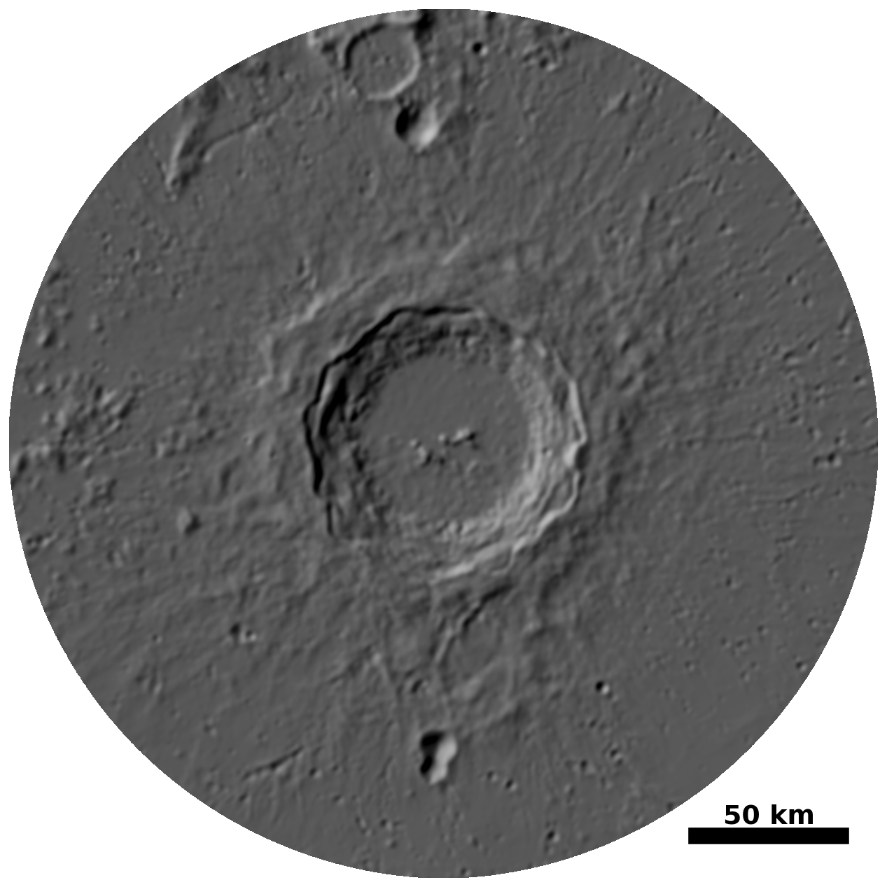
Many applications of Cratermaker could potentially use real digital elevation model (DEM) data as the starting surface topography. The "datasurface" Surface type is designed for this purpose. It is based on the "hireslocal" surface type, but will construct a surface and initialize it based on a DEM. When using the Moon as a target body, Cratermaker can fetch DEM data from the NASA PDS automatically, and only requires a minimum of the local_location and local_radius arguments.

By default, it will find data file that contains approximately \(10^6\) faces. Passing an optional argument pix will override this default behavior and it will attempt to find a DEM file that comes closest to matching the requested pixel size. Optionally, the user can also pass in one or more file paths or URLs to DEM files using the dem_file_list argument. Like “hireslocal,” this surface will contain a local region and a global superdomain.

The superdomain will be initialized using a low resolution global DEM, or optionally a file path or URL to a DEM file can be passed in using the superdomain_dem_file argument.

How DataSurface chooses lunar DEM files

When the target body is the Moon and you do not provide explicit DEM files, DataSurface will automatically select appropriate LOLA/SLDEM products from the NASA PDS based on the requested region and resolution.

Local-region DEM (dem_file_list)

If dem_file_list is not provided, the class chooses DEM sources as follows:

1. Pick a target resolution If pix is not given, a default pixel size is computed to yield roughly \(10^6\) faces in the local region. If pix is given, it is treated as the desired meters-per-pixel for the local DEM.

2. Compute geographic coverage The code computes a lon/lat bounding box for the local circular region (centered at local_location with radius local_radius). If the region reaches a pole, longitudes are treated as global (-180 to 180).

3. Choose projection family (polar vs. cylindrical) A target angular resolution (pixels/degree) is estimated from pix and the lunar radius. If the implied resolution is high (greater than ~10 pix/deg) and the region extends beyond lat = 60° (North or South), the polar LOLA products are used. Otherwise, cylindrical products are used.

4. Select the closest available dataset resolution - Cylindrical: chooses the nearest available product from [4, 16, 64, 128, 256, 512] pix/deg. For low-resolution global products (<256 pix/deg), a single global file covers the domain. For high-resolution tiled products (≥256 pix/deg), the tile containing the center is selected, and additional neighboring tiles are added as needed to cover the bounding box corners. - Polar: chooses the closest available meters-per-pixel product that covers the requested latitude range (datasets have minimum-latitude coverage thresholds that depend on the product).

Global superdomain DEM (superdomain_dem_file)

If superdomain_dem_file is not provided (and the superdomain has been defined), the class:

1. Computes a coarser target pixel size from the local resolution and superdomain_scale_factor (with a minimum corresponding to ~128 pix/deg globally), then

2. Uses the same selection logic as above (polar vs. cylindrical) to pick a suitable global DEM file for initializing elevations outside the local region.

Overriding file selection

You can bypass all automatic dataset selection by providing:

• dem_file_list: one or more file paths or URLs for the local region DEM(s)

• superdomain_dem_file: a file path or URL for the global DEM.

Cratermaker uses rasterio to read DEM files, and so any format supported by rasterio should work (e.g., GeoTIFF, IMG, etc.).

Extracting a local subsection of the surface

Many of the operations that Cratermaker does on a surface only affect a small portion of the full grid at a time. The Surface class has a tool that is used to efficiently extract a local subsection of a given surface without making a copy in memory. This is done by creating a LocalSurface object, which is a view of the original surface that contains the faces, nodes, and edges within a specified radius of a given location. The LocalSurface object can be used to perform operations on this local region rather than on the full set of faces, nodes, and edges. To generate a LocalSurface, you can use the extract_region() method of the Surface class. This method takes two arguments: location, which is a tuple of (longitude, latitude) in degrees, and region_radius, which is the radius of the region in meters. This will return a LocalSurface object that contains all faces within a specified radius, plus a buffer of surrounding faces. All nodes and edges associated with the faces inside the primary local region are included, but only nodes associated with the buffer faces are included, but not edges (see the diagram above). This is done to prevent array out of bounds issues when performing operations that require neighboring faces across included edges, as is done when computing topographic diffusion calculations.

For instance, suppose we’d like to extract a 16 km radius region at the south pole of the Moon:

In [10]: surface=Surface.maker()
Creating a new grid
Generating a mesh with icosphere level 8.

In [11]: print(surface)
<IcosphereSurface>
Target: Moon
Grid File: surface/grid.nc
Number of faces: 655362
Number of nodes: 1310720
Grid Level: 8
Effective pixel size: 7.602 km +/- 319.2 m


In [12]: region=surface.extract_region(location=(0,-90),region_radius=16e3)

In [13]: print(region)
<LocalSurface>
Location: 0.00°, -90.00°
Region Radius: 16.00 km
Number of faces: 33
Number of nodes: 88

As we can see, this selects only 33 of the full 655362 faces, which is a significant reduction in the number of faces and nodes that need to be processed. All faces with their centers interior to circle defined by location and region_radius are included, as well as their associated edges and nodes (highlighted in the diagram above). In addition, the region will also contain a “buffer” of all faces that surround the outermost border of the local region, such that any operations that require neighboring faces across included edges or nodes can have access to them.

Note

The "hireslocal" Surface type contains a built-in attribute called local, which represents the high resolution region of the surface. In addition, when extract_region() is called on a “hireslocal” surface, it will return a special LocalHiResLocalSurface object that contains within it an additional object called local_overlap. This is a view of only the portion of the extracted region that overlaps the high resolution region (or None if there is no overlap).

Using a Surface object

Once you have either a Surface or LocalSurface object, you are now able to perform numerous surface-related computations.

• extract_region(): Extracts a local region of the surface, which is useful for performing operations on a small portion of the surface without affecting the full surface. This returns a LocalSurface object.

• add_data(): Adds a new data variable that is associated with either faces (default) or nodes of the surface.

• update_elevation(): Updates the elevation data of the surface using the new_elevation argument. The data is added to the existing elevation data by default, unless the user specifies overwrite=True.

• apply_diffusion(): Applies diffusive degradation to the surface, which is a process that smooths out the surface by averaging the elevations of neighboring faces. This is useful for simulating the effects of erosion over time.

• slope_collapse(): Applies diffusion only to surfaces that are steeper than a given threshold given by the argument critical_slope_angle, which is set to 35 degrees by default (a typical value for the angle of repose).

• apply_noise(): Applies tubulence-style simplex noise to the surface. This can be useful for generating realistic surface features, such as hills and valleys. The noise is applied to the elevation data of the surface.

• calculate_face_and_node_distances(): Returns one array for distances between a point and all faces, and another array with distances between that point and all nodes.

• calculate_face_and_node_bearings(): Returns two arrays: Bearings (direction in degrees) between a point and all faces, Bearing between a point and all nodes.

• find_nearest_face(): Returns the index of the face that is closest to a given point.

• find_nearest_node(): Returns the index of the node that is closest to a given point.

• interpolate_node_elevation_from_faces(): Some operations only affect faces, and so this method can be used to interpolate the elevation of nodes from the face elevations.

• elevation_to_cartesian(): Convert elevation values to Cartesian coordinates. This is a basic utility function that takes the cartesian positions of the surface of a sphere and elevation values and returns the Cartesian coordinates of the surface with the elevations applied. This is used because the mesh is never altered in Cratermaker, but rather the elevations are applied to the mesh when it is visualized.

• get_random_location_on_face(): Given a face index, this method will return a random location on that face. This is used to generate craters on a surface, as some surfaces have highly variable faces and therefore production functions must be evaluated on a face-by-face basis.

Note

The LocalSurface object comes with distances and bearings from the center of the local region pre-computed. See below:

In [14]: region=surface.extract_region(location=(205,45),region_radius=10e3)

In [15]: print(f"Region face distances:\n{region.face_distance}")
Region face distances:
[ 9875.62158822  8359.08613442 15866.73929187  9860.95218414
 12882.00753763 13313.98819277 16823.31984602 15148.4839375
  5089.30240275 16686.72288194 12821.57156235 16872.20557816
 17439.51146968  9949.44440087  5964.15127258 16809.44514818
 13906.92341485  3076.86061662 18253.04695568 10802.09822748]

In [16]: print(f"Region face bearings:\n{region.face_bearing}")
Region face bearings:
[263.3601638   16.0979079   89.82530658 157.72344712 305.25452333
 223.11242812 279.75274061  33.59598695 312.59513719   5.52979319
 339.66095662 250.15336587  60.35228351  66.04310758 210.60444675
 141.28869633 189.62881453 100.23728128 165.89432969 114.8435246 ]

Examples

Extracting a local subset of the grid

Suppose we wish to extract a 10 km radius local region of the surface of the Moon centered at 45° N latitude, 205° E longitude:

In [17]: surface=Surface.maker()
Creating a new grid
Generating a mesh with icosphere level 8.

In [18]: region=surface.extract_region(location=(205,45), region_radius=10e3)

In [19]: print(f'Local region: {region}')
Local region: <LocalSurface>
Location: -155.00°, 45.00°
Region Radius: 10.00 km
Number of faces: 20
Number of nodes: 57

The region object now contains a view of all faces (along with their corresponding nodes and edges) of a local subset of the grid. Because it is a view of the surface not a copy, it allows for fast computation on small portions of the full grid..

Distances and bearings

The LocalSurface object has two attributes called face_distance and face_bearing (and also node_distance and node_bearing), which are pre-computed distances and bearings from the center of the local region to all faces (nodes). This is useful for quickly accessing these values without having to compute them yourself.

In [20]: print(f'Face distances from center of local region: {region.face_distance}')
Face distances from center of local region: [ 9875.62158822  8359.08613442 15866.73929187  9860.95218414
 12882.00753763 13313.98819277 16823.31984602 15148.4839375
  5089.30240275 16686.72288194 12821.57156235 16872.20557816
 17439.51146968  9949.44440087  5964.15127258 16809.44514818
 13906.92341485  3076.86061662 18253.04695568 10802.09822748]

In [21]: print(f'Face bearings from center of local region: {region.face_bearing}')
Face bearings from center of local region: [263.3601638   16.0979079   89.82530658 157.72344712 305.25452333
 223.11242812 279.75274061  33.59598695 312.59513719   5.52979319
 339.66095662 250.15336587  60.35228351  66.04310758 210.60444675
 141.28869633 189.62881453 100.23728128 165.89432969 114.8435246 ]

We can see that the local region contains points outside of the 10 km region. We can see that this region contains 20 faces and 25 nodes, but only 7 of the faces actually lie within the 10 km local region, while the other 13 are part of the buffer. From here, we can perform many of the calculations as seen in the list above.

We can also calculate these for any arbitrary point within the local region (or full surface) using the methods calculate_face_and_node_distances() and calculate_face_and_node_bearings(). For instance, suppose we want to find the distances and bearings between a point at (205,45) and all faces and nodes in the local region:

In [22]: face_distance, node_distance=region.calculate_face_and_node_distances(location=(205,45))

In [23]: print(f'Distances betwen location (205,45) and faces :{face_distance}')
Distances betwen location (205,45) and faces :[ 9875.62158822  8359.08613442 15866.73929187  9860.95218414
 12882.00753763 13313.98819277 16823.31984602 15148.4839375
  5089.30240275 16686.72288194 12821.57156235 16872.20557816
 17439.51146968  9949.44440087  5964.15127258 16809.44514818
 13906.92341485  3076.86061662 18253.04695568 10802.09822748]

In [24]: print(f'Distances betwen location (205,45) and nodes :{node_distance}')
Distances betwen location (205,45) and nodes :[19771.00775882 21389.54457962 19951.60985076 14504.1805421
  9020.99468831  5237.79291219  1768.22722877  5252.77041231
 14750.06024199 12285.20450267 15105.88089176  6965.42435014
 22811.84951808 22345.08636317 12301.13886375 21401.90804946
  9592.14390261 14962.11013764 17850.56488892  3708.38074022
  8218.20255989 13012.52599312 12175.69552653 18448.52611073
 20520.06463349  9329.30480112 17140.74009023 16829.75872035
 19963.56385549 16736.26603506 17452.05464756 20757.99191701
 14369.49366246 11215.08564406  7690.39968393  5902.09498583
 13497.27591065 10748.88780693 18246.94494406 17628.89840045
 16927.3626356  20045.8995352  12528.9876261  21346.62233282
 14519.47172295 18058.13901357 21097.67981161 21666.66601396
 17891.83724341 19665.67943804 21259.65240107 17854.4565761
 18527.11405992 13758.41664206 15518.95195962  9320.88365039
 10552.24682596]

With this method, two arrays are returned where the first array gives us an array of distances between the input location and all of the faces, and the second array returns the distances from the input locaion and all of the nodes. It is best to use this method on smaller regions due to the size of the arrays if used on entire surface. We can do a similar calculation, but rather finding the distances between a location and the faces and nodes, we find the bearings:

In [25]: face_bearing, node_bearing =region.calculate_face_and_node_bearings(location=(205,45))

In [26]: print(f'Bearings betwen location (205,45) and faces :{face_bearing}')
Bearings betwen location (205,45) and faces :[263.3601638   16.0979079   89.82530658 157.72344712 305.25452333
 223.11242812 279.75274061  33.59598695 312.59513719   5.52979319
 339.66095662 250.15336587  60.35228351  66.04310758 210.60444675
 141.28869633 189.62881453 100.23728128 165.89432969 114.8435246 ]

In [27]: print(f'Bearings betwen location (205,45) and nodes :{node_bearing}')
Bearings betwen location (205,45) and nodes :[152.59348158 143.79339469 130.52935616 156.16869948 291.40936048
 162.03127303 246.74421739 259.12854102 126.05519426 136.92504234
 106.88301201 132.32150395 163.25861926 172.18983684 284.11862179
 277.2447301  322.27702138 322.49970171  75.45237509  14.13647775
 343.49861188  16.65713326   0.92013653 102.82317828  89.44235704
 235.49885671 312.49004074 295.64886751 290.50438406 349.52068531
 337.85489748 358.58093242  73.04171013  90.52583133  92.94800274
  48.7869727   51.10157712  40.42370296  45.58794111 216.59370296
 234.32771539 239.53614811 243.5701873  254.01191364 264.89005967
 264.96409027  51.74781933  66.09942849  20.48024159  29.8702336
   8.16781131 180.65332141 191.6404801  170.26722957 206.72150263
 185.62774682 204.93477683]

As you can see from above, we recieve two arrays, which are the same sizes as the previous examples. However, they now tell us the “initial bearing” (the direction relative to due North) between a point and all faces and all nodes.

Finding a face index

Suppose we would like to find a face correspnding to a particulal location. We can do the following:

In [28]: face_index=surface.find_nearest_face(location=(205,45))

In [29]: print(f'Nearest face to (205,40): {face_index}')
Nearest face to (205,40): 579207

As seen above, we recieve an integer that gives us the index to the nearest face. One caveat is that this method will return the index of the face in which its center is the closest to the input location. Due to the shapes of the faces, this may or may not correspond to the face that contains the input location. However, it should correspond to at least one of the faces that borders the one containing the input location. A diagram of this is seen below:

In the diagram above, we observe a point located within face \(f_0\) with a distance \(d_0\) from the center of the face. A neighboring face, \(f_1\), is adjacent to \(f_0\) and has a corresponding distance, \(d_1\), to its center, where \(d_0 > d_1\). Hence, the find_nearest_face method will return \(f_1\) as the closest face due to \(d_1\) being a shorter distance. You can view which faces these are using one of the built-in connectivity arrays. In this case, face_face_connectivity contains the array of faces that are connected to a particular face:

In [30]: print(f'Neighboring faces of {face_index} include: {surface.face_face_connectivity[face_index]}')
Neighboring faces of 579207 include: [579204 144917 579141 579209 144904 579196]

There are corresponding methods for finding the nearest node, as well as connectivity arrays for nodes, such as node_face_connectivity (faces associated with each node) and face_node_connectivity (nodes associated with each face).

Note

Due to the variable number of nodes and edges associated with each face, there will sometimes be unused elements of the connectivity arrays. These are set to a large negative number, and so filtering out only indices greater than or equal to 0 will give you the valid indices.

Converting elevation to Cartesian coordinates

Cratermaker saves the face and node elevations independently of the mesh geometry. Suppose you want to visualize the surface with the elevations applied. You can use the elevation_to_cartesian() method to convert the elevations to Cartesian coordinates. This method takes one argument, element, which can either be “face” or “node”. The method will return an (n, 3) array of Cartesian coordinates, where n is the number of faces or nodes, depending on the value of element.

In [31]: region = surface.extract_region(location=(0,0), region_radius=10e3)

In [32]: cartesian = region.elevation_to_cartesian(element='face')

In [33]: print(cartesian)
[[ 1.73753000e+06 -1.25589390e-13  0.00000000e+00]
 [ 1.73746289e+06 -1.25589363e-13 -1.52711111e+04]
 [ 1.73746289e+06 -1.25589363e-13  1.52711111e+04]
 [ 1.73744748e+06  1.45852811e+04 -8.60454234e+03]
 [ 1.73744748e+06 -1.45852811e+04 -8.60454234e+03]
 [ 1.73744748e+06  1.45852811e+04  8.60454234e+03]
 [ 1.73744748e+06 -1.45852811e+04  8.60454234e+03]
 [ 1.73751269e+06  1.25589363e-13 -7.75672851e+03]
 [ 1.73751269e+06 -1.25589363e-13  7.75672851e+03]
 [ 1.73750965e+06  7.33012990e+03 -4.12061614e+03]
 [ 1.73747342e+06  7.25525700e+03 -1.19985013e+04]
 [ 1.73750965e+06 -7.33012990e+03 -4.12061614e+03]
 [ 1.73747342e+06 -7.25525700e+03 -1.19985013e+04]
 [ 1.73750965e+06  7.33012990e+03  4.12061614e+03]
 [ 1.73747342e+06  7.25525700e+03  1.19985013e+04]
 [ 1.73746941e+06  1.45106075e+04 -3.76768328e-13]
 [ 1.73750965e+06 -7.33012990e+03  4.12061614e+03]
 [ 1.73747342e+06 -7.25525700e+03  1.19985013e+04]
 [ 1.73746941e+06 -1.45106075e+04  3.76768328e-13]]

This could be used to visualize the surface using a 3D plotting library, such as Matplotlib or Plotly. The Cartesian coordinates will have the elevations applied, so you can see the topography of the surface.

See also

• Surface for the API reference

• Example Gallery for more examples of using the Surface component in the Gallery section.