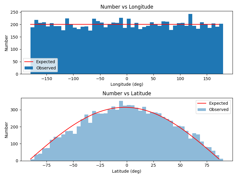
Plot a distribution of random locations

By David Minton and Dennise Valadez

This example demonstrates the generation of random impact locations.

import matplotlib.pyplot as plt
import numpy as np

from cratermaker import Projectile

# Create a projectile
proj = Projectile(mean_velocity=5000, density=3000)

# Using projectile for sampling data
size = 10000
locations = [proj.new_projectile().location for _ in range(size)]

# Obtain longitudes and latitudes from projectile - but this is not accurate and doesnt work
lons = np.array([loc[0] for loc in locations])
lats = np.array([loc[1] for loc in locations])

# Bins
bins = 50

# Longitude histogram
observed_counts_lon, bins_lon_deg = np.histogram(lons, bins=bins, range=(-180, 180.0))
expected_count_lon = size // bins

# Latitude histogram
observed_counts_lat, bins_lat_deg = np.histogram(lats, bins=bins, range=(-90, 90))
bins_lat = np.deg2rad(bins_lat_deg)
area_ratio = np.sin(bins_lat[1:]) - np.sin(bins_lat[:-1])
total_area = np.sin(np.pi / 2) - np.sin(-np.pi / 2)
expected_count_lat = size * area_ratio / total_area

# Bar widths
bar_width_lon = np.diff(bins_lon_deg)
bar_width_lat = np.diff(bins_lat_deg)

# Plotting
fig, axs = plt.subplots(2, 1, figsize=(8, 6))

# Longitude plot
axs[0].bar(
    bins_lon_deg[:-1],
    observed_counts_lon,
    width=bar_width_lon,
    align="edge",
    label="Observed",
)
axs[0].plot(
    bins_lon_deg[:-1],
    [expected_count_lon] * len(bins_lon_deg[:-1]),
    color="red",
    label="Expected",
)
axs[0].set_xlabel("Longitude (deg)")
axs[0].set_ylabel("Number")
axs[0].legend()
axs[0].set_title("Number vs Longitude")

# Latitude plot
axs[1].bar(
    bins_lat_deg[:-1],
    observed_counts_lat,
    width=bar_width_lat,
    align="edge",
    alpha=0.5,
    label="Observed",
)
axs[1].plot(bins_lat_deg[:-1], expected_count_lat, label="Expected", color="red")
axs[1].set_xlabel("Latitude (deg)")
axs[1].set_ylabel("Number")
axs[1].legend()
axs[1].set_title("Number vs Latitude")

plt.tight_layout()
plt.show()