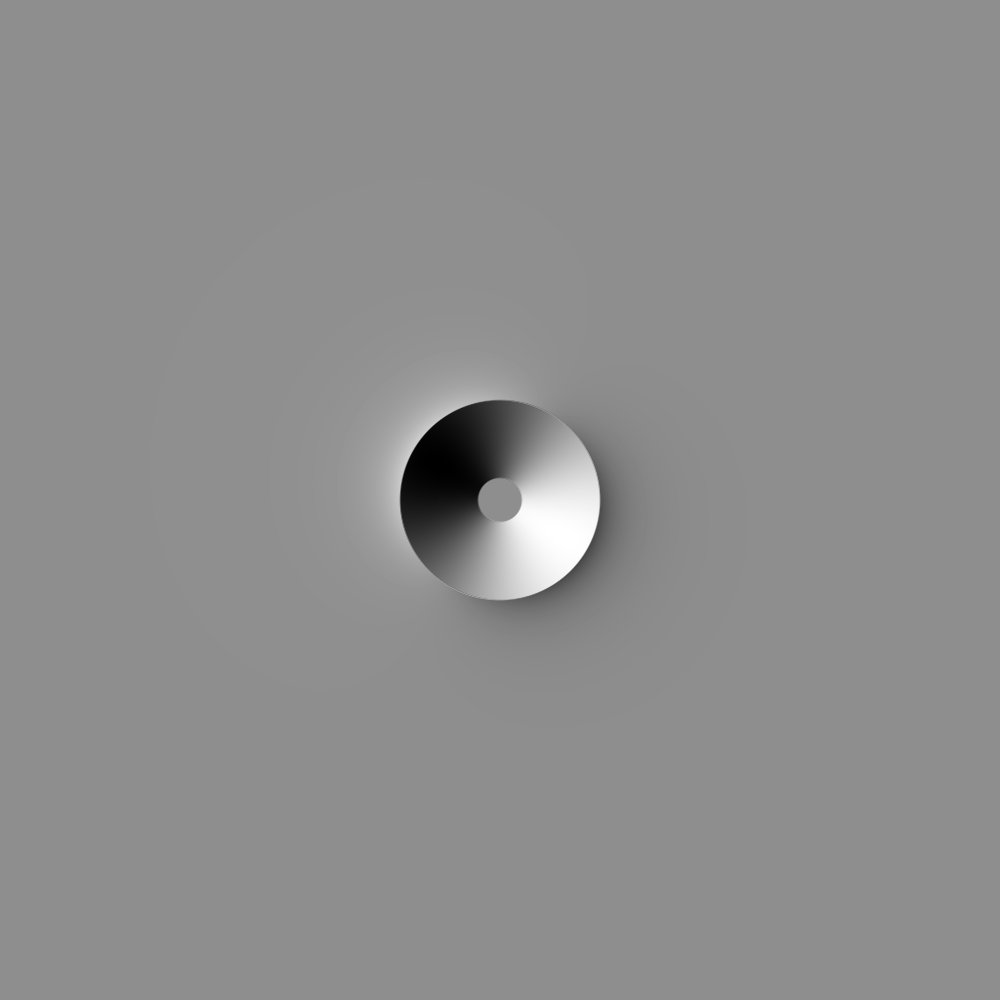
Create a shaded topographic representation of a crater

By David Minton

This example showcases how to create a crater and ejecta profile using the “basicmoon” morphology model from the Cratermaker and visual its topography. This will mimic how CTEM generates a test crater, though it is much simpler to run than that venerable old Fortran-based beast of a code!. The crater is created with a radius of 1 km. The hill shade uses the same settings that CTEM uses.

Note, that this example is rather more complex than it really needs to be. In practice, the Morphology object is always associated with a Surface object, which contains its own set of methods for visualizing the surface morphology. For this example, we are bypassing the Surface object functionality entirely and generating our own grid for illustration purposes. Example 1.1-visualize_one_crater.py demonstrates a more “typical” approach.

Creating a new grid
Generating a mesh with icosphere level 4.

import numpy as np

from cratermaker import Crater, Morphology

# Because we are not explicitly passing a Surface object, the Morphology constructor will generate a default surface. We pass the "simdir" and "gridlevel" arguments to control the Surface generation, even though we don't make use of it directly here.
morphology = Morphology.maker("basicmoon", simdir="simdata-4_1", gridlevel=4)
crater = Crater.maker(radius=1.0e3)

# Generate 1000x1000 grid centered at (0, 0)
gridsize = 1000
extent = 5e3  # +/- extent in meters
pix = 2 * extent / gridsize  # pixel size in meters
x = np.linspace(-extent, extent, gridsize)
y = np.linspace(-extent, extent, gridsize)
xx, yy = np.meshgrid(x, y)

# Compute radial distance from center
r = np.sqrt(xx**2 + yy**2)

# Compute crater and ejecta profiles
crater_elevation = morphology.crater_profile(crater, r)
ejecta_elevation = morphology.ejecta_profile(crater, r)

# Combine into a total DEM
dem = crater_elevation + ejecta_elevation


def plot(dem, pix):
    import matplotlib.pyplot as plt
    from matplotlib.colors import LightSource

    dpi = 300
    gridsize = dem.shape[0]
    # Create hillshade
    azimuth = 300.0  # user['azimuth']
    solar_angle = 20.0  # user['solar_angle']
    height = gridsize / dpi
    width = gridsize / dpi
    fig = plt.figure(figsize=(width, height), dpi=dpi)
    ax = plt.axes([0, 0, 1, 1])

    ls = LightSource(azdeg=azimuth, altdeg=solar_angle)
    hillshade = ls.hillshade(dem, dx=pix, dy=pix, fraction=1)

    # Plot the shaded relief
    ax.imshow(
        hillshade,
        interpolation="nearest",
        cmap="gray",
        vmin=0.0,
        vmax=1.0,
        extent=(-extent, extent, -extent, extent),
    )
    plt.axis("off")
    plt.show()


plot(dem, pix)